Losses

A collection of losses including:

• Spectral log magnitude loss
• Spectral convergence loss
• Wasserstein loss

---

wasserstein_1d

 wasserstein_1d (u_values, v_values, u_weights=None, v_weights=None, p=1,
                 require_sort=True)

*This is a port of the wasserstein_1d function from POT in JAX. Computes the 1 dimensional OT loss [15] between two (batched) empirical distributions

.. math: OT_{loss} = _0^1 |cdf_u^{-1}(q) - cdf_v^{-1}(q)|p dq

It is formally the p-Wasserstein distance raised to the power p. We do so in a vectorized way by first building the individual quantile functions then integrating them.

This function should be preferred to emd_1d whenever the backend is different to numpy, and when gradients over either sample positions or weights are required.*

	Type	Default	Details
u_values
v_values
u_weights	NoneType	None
v_weights	NoneType	None
p	int	1
require_sort	bool	True
Returns	cost: float/array-like, shape (…)		the batched EMD

---

quantile_function

 quantile_function (qs, cws, xs)

Computes the quantile function of an empirical distribution

	Type	Details
qs
cws
xs
Returns	q: array-like, shape (…, n)	The quantiles of the distribution

---

compute_mag

 compute_mag (x:jax.Array)

	Type	Details
x	Array	(b, t)
Returns	Array

---

spectral_wasserstein

 spectral_wasserstein (x, y, squared=True, is_mag=False)

---

log_mag_loss

 log_mag_loss (pred:jax.Array, target:jax.Array, eps:float=1e-10,
               distance:str='l1')

Spectral log magtinude loss but for a fft of a signal See Arik et al., 2018

	Type	Default	Details
pred	Array		complex valued fft of the signal
target	Array		complex valued fft of the signal
eps	float	1e-10
distance	str	l1

---

log_mag

 log_mag (x:jax.Array, eps:float=1e-10)

phase = 0.0
omegas = jax.random.uniform(jax.random.PRNGKey(0), shape=(10,)) * 100
mag = 0.99


def osc_bank(t, omegas):
    return mag * jnp.sin(omegas[..., None] * jnp.pi * 2 * t[None] + phase)

t = jnp.linspace(0, 1, 1000)
gt_osc_values = osc_bank(t, omegas)
# print(gt_osc_values)
print(gt_osc_values.shape)

(10, 1000)

a = jax.vmap(spectral_wasserstein)(gt_osc_values, gt_osc_values)
print(a)

[0. 0. 0. 0. 0. 0. 0. 0. 0. 0.]

def loss_fn(omega):
    pred_osc_values = osc_bank(t, omega)
    x_fft = compute_mag(gt_osc_values)
    y_fft = compute_mag(pred_osc_values)
    l2_mag_loss = jnp.mean((x_fft - y_fft) ** 2)
    return l2_mag_loss


def ot_loss_fn(omega):
    pred_osc_values = osc_bank(t, omega)

    ot_loss = jnp.mean(
        jax.vmap(spectral_wasserstein)(gt_osc_values, pred_osc_values),
    )
    return ot_loss

x_fft = compute_mag(gt_osc_values) ** 2
plt.plot(x_fft[:5].T)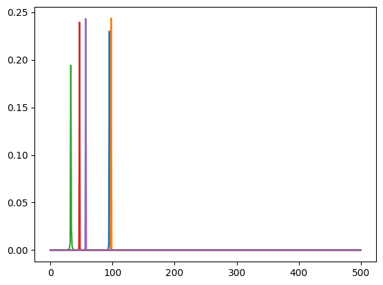

ranges = jnp.linspace(-50, 50, 100)
omegas_scan = omegas + ranges[:, None]

# print(omegas_scan.shape)
loss, grad = jax.vmap(jax.value_and_grad(loss_fn))(omegas_scan)
loss_ot, grad_ot = jax.vmap(jax.value_and_grad(ot_loss_fn))(omegas_scan)

print(loss.shape, loss.dtype)
print(loss_ot.shape, loss_ot.dtype)
plt.plot(ranges, loss_ot)

(100,) float32
(100,) float32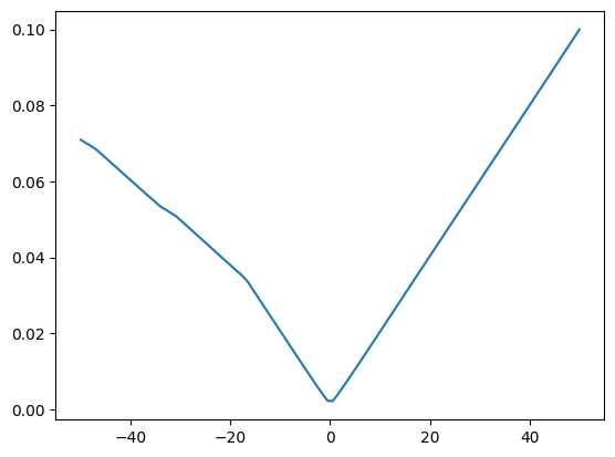

omegas_gt = jax.random.uniform(jax.random.PRNGKey(0), shape=(10,)) * 1000
omegas_pred = omegas_gt * 1

pred_osc_values = osc_bank(t, omegas_pred).mean(axis=0)
gt_osc_values = osc_bank(t, omegas_gt)

x_mag = compute_mag(gt_osc_values.mean(axis=0))
y_mag = compute_mag(pred_osc_values)

plt.semilogx(x_mag)
plt.semilogx(y_mag)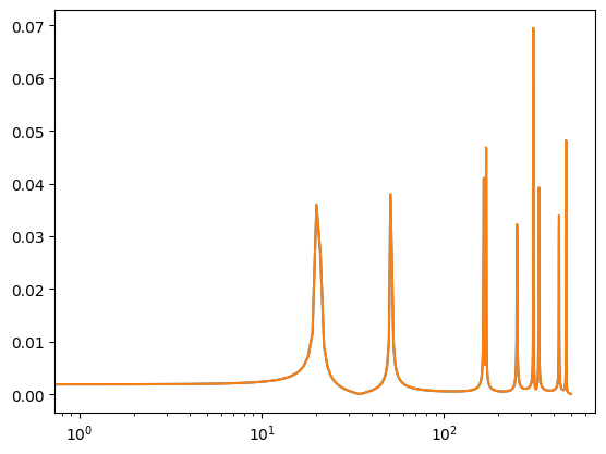

---

spectral_convergence_loss

 spectral_convergence_loss (pred:jax.Array, target:jax.Array)

Spectral convergence loss but for a fft of a signal See Arik et al., 2018

	Type	Details
pred	Array	magnitude of the fft of the predicted signal
target	Array	magnitude of the fft of the target signal