Non-linear models

The non-linear models are also similar to simulate. We add a non-linear to the equation:

\[\begin{equation} \rho \ddot{w} + \left(d_1 + d_3 \Delta\right)\dot{w} + (D \Delta \Delta - T_0 \Delta) w = f_{\text{ext}} - f_{\text{nl}}, \end{equation}\]

where \(f_{\text{nl}}\) is the non-linear term. Again we get damped harmonic oscillators:

\[\begin{equation} \ddot{q}_{\mu} + 2\gamma_{\mu}\dot{q}_{\mu} + \omega_{\mu}^2 q_{\mu} = \bar{f}_{\text{ext},\mu} - \bar{f}_{\text{nl},\mu}, \end{equation}\]

where \(\bar{f}_{\text{nl},\mu}\) is the non-linear term in modal space. This term differs depending on the type of non-linearity and whether we are simulating a string, membrane or plate.

Tension modulated string

For tension-modulated strings the non-linear term expanded in modal coordinates is given by:

\[\begin{equation} \bar{f}_{nl} = \tau \sum_{\mu} \frac{\lambda_{\mu} q_{\mu}^2}{||\Phi_{\mu}||^2}, \end{equation}\]

where \(\tau\) is:

\[\begin{equation} \tau = \frac{E A}{2 L} \end{equation}\]

First, we set up the parameters for the string.

n_modes = 50
n_steps = 44100
sample_rate = 44100
dt = 1.0 / sample_rate
excitation_position = 0.2
readout_position = 0.5
initial_deflection = 0.04
n_gridpoints = 101  # number of gridpoints for evaluating the eigenfunctions
string_params = StringParameters()

Get the eigenpairs and the initial condition

lambda_mu = string_eigenvalues(n_modes, string_params.length)
wn = np.sqrt(lambda_mu)
grid = np.linspace(0, string_params.length, n_gridpoints)
K = string_eigenfunctions(wn, grid)


u0_modal = create_pluck_modal(
    lambda_mu,
    pluck_position=excitation_position,
    initial_deflection=initial_deflection,
    string_length=string_params.length,
)
u0 = inverse_STL(K, u0_modal, string_params.length)
fig, ax = plt.subplots(1, 1, figsize=(6, 2))
ax.plot(grid, u0)
ax.set_xlabel("Position (m)")
ax.set_ylabel("Deflection (m)")
ax.set_title("Initial deflection of the string")
ax.grid(True)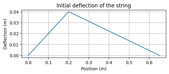

Define the non-linear term and integrate in time

gamma2_mu = damping_term(string_params, lambda_mu)
omega_mu_squared = stiffness_term(string_params, lambda_mu)

string_tau = string_tau_with_density(string_params)
string_norm = string_params.length / 2

# include the norm and lambda_mu to make it more compact
string_tau = string_tau * lambda_mu / string_norm

nl_fn = make_tm_nl_fn(lambda_mu, string_tau)
_, modal_sol = solve_tf_initial_conditions(
    gamma2_mu,
    omega_mu_squared,
    u0=u0_modal,
    v0=jnp.zeros_like(u0_modal),
    dt=dt,
    n_steps=n_steps,
    nl_fn=nl_fn,
)

# transpose to have modes in the first dimension
modal_sol = modal_sol.T

print(modal_sol.shape)

(50, 44100)

mu = np.arange(1, n_modes + 1)  # mode indices

readout_weights = evaluate_string_eigenfunctions(
    mu,
    readout_position,
    string_params,
)

# at a single point
u_readout = readout_weights @ modal_sol

# at all points
sol = inverse_STL(K, modal_sol, string_params.length)

display(Audio(u_readout, rate=sample_rate))
fig, ax = plt.subplots(1, 1, figsize=(6, 2))
ax.plot(u_readout)
ax.set_xlabel("Sample")
ax.set_ylabel("Deflection (m)")
ax.set_title("Deflection of the string at a single point")
ax.set_xlim(-2, sample_rate // 10)
ax.grid(True)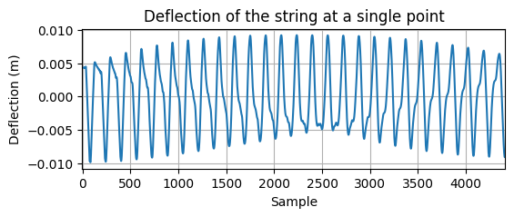

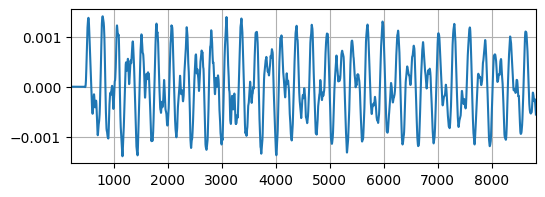
Tension modulated plate

The tension-modulated plate works just like the string we saw earlier, same non-linear term, but with a different \(\tau\) value:

\[ \tau = \frac{E h}{2 L_x L_y (1 - \nu^2)} \]

Define the parameters for the plate

n_modes_x = 15
n_modes_y = 15
n_modes = n_modes_x * n_modes_y
n_steps = 44100
sample_rate = 44100
dt = 1.0 / sample_rate
excitation_duration = 1.0  # seconds
excitation_amplitude = 40
force_position = (0.05, 0.05)
readout_position = (0.1, 0.1)
plate_params = PlateParameters(
    Ts0=0.0,
    d1=1e-4,
    d3=1e-2,
)

Get the eigenpairs and the excitation

wnx, wny = plate_wavenumbers(
    n_modes_x,
    n_modes_y,
    plate_params.l1,
    plate_params.l2,
)
lambda_mu_2d = plate_eigenvalues(wnx, wny)
n_gridpoints_x = 101
n_gridpoints_y = 151
x = np.linspace(0, plate_params.l1, n_gridpoints_x)
y = np.linspace(0, plate_params.l2, n_gridpoints_y)
K = plate_eigenfunctions(wnx, wny, x, y)

# Sort the eigenvalues and get the indices
indices = np.argsort(lambda_mu_2d.ravel())
ky_indices, kx_indices = np.unravel_index(indices, lambda_mu_2d.shape)
ky_indices, kx_indices = ky_indices + 1, kx_indices + 1
selected_indices = np.stack([kx_indices, ky_indices], axis=-1)
lambda_mu = np.sort(lambda_mu_2d.reshape(-1))

rc = create_1d_raised_cosine(
    duration=excitation_duration,
    start_time=0.010,
    end_time=0.012,
    amplitude=excitation_amplitude,
    sample_rate=sample_rate,
)

weights_at_ex = (
    evaluate_rectangular_eigenfunctions(
        selected_indices,
        force_position,
        params=plate_params,
    )
    / plate_params.density
)

weights_at_readout = evaluate_rectangular_eigenfunctions(
    selected_indices,
    readout_position,
    params=plate_params,
)

modal_excitation = np.outer(rc, weights_at_ex)

Define the non-linear term and integrate in time

gamma2_mu = damping_term(
    plate_params,
    lambda_mu,
)
omega_mu_squared = stiffness_term(
    plate_params,
    lambda_mu,
)

plate_tau = (plate_params.E * plate_params.h) / (
    2 * plate_params.l1 * plate_params.l2 * (1 - plate_params.nu**2)
)
plate_tau = plate_tau / plate_params.density
plate_norm = 0.25 * plate_params.l1 * plate_params.l2

plate_tau = plate_tau * lambda_mu / plate_norm

nl_fn = make_tm_nl_fn(lambda_mu, plate_tau)

_, modal_sol = solve_tf_excitation(
    gamma2_mu,
    omega_mu_squared,
    modal_excitation,
    dt,
    nl_fn=nl_fn,
)

modal_sol = modal_sol.T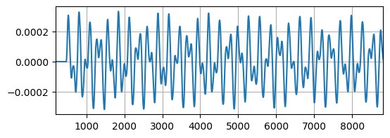

Von Karman plate

In the Von Karman plate we have a different non-linear term:

\[\begin{equation} \bar{f}_{nl} = \frac{E S_w}{2 \rho} \sum_{p, q, r}^n \frac{H_{q, r}^n C_{p, n}^s}{\zeta_n^4} q_p q_q q_r, \end{equation}\]

We will use the same parameters as in the tension-modulated plate above but now we need the coupling coefficients (assuming simply supported boundary conditions). Calculating the coupling coefficients can take a while, so we will only use 10 in-plane modes and all transverse modes. We will also set \(S_w = ||\Phi||^2\) and increase the excitation amplitude to make the coupling effect more noticeable

Integrate in time. This is fast however with more modes it will take longer. In any case, this will take longer than the tension-modulated plate.

gamma2_mu = damping_term(
    plate_params,
    lambda_mu,
)
omega_mu_squared = stiffness_term(
    plate_params,
    lambda_mu,
)

nl_fn = make_vk_nl_fn(H1_scaled)

_, modal_sol = solve_tf_excitation(
    gamma2_mu,
    omega_mu_squared,
    modal_excitation * amplitude_scaling,
    dt,
    nl_fn=nl_fn,
)

modal_sol = modal_sol.T