Linear models

For the linear models we want to solve the following equation:

\[\begin{equation} \rho \ddot{w} + \left(d_1 + d_3 \Delta\right)\dot{w} + (D \Delta \Delta - T_0 \Delta) w = f_{\text{ext}}, \end{equation}\]

which in modal coordinates \(q_{\mu}\) results in uncoupled damped harmonic oscillators:

\[\begin{equation} \ddot{q}_{\mu} + 2\gamma_{\mu}\dot{q}_{\mu} + \omega_{\mu}^2 q_{\mu} = \bar{f}_{\text{ext},\mu}, \end{equation}\]

where the coefficients are given by:

\[\begin{align} \omega_{\mu}^2 &= \frac{D\lambda_{\mu}^2 - T_0\lambda_{\mu}}{\rho},\\ \gamma_{\mu} &= \frac{d_1 + d_3\lambda_{\mu}}{2\rho}. \end{align}\]

String

Some parameters for the string

n_modes = 50
n_steps = 44100
sample_rate = 44100
dt = 1.0 / sample_rate
excitation_position = 0.2
readout_position = 0.5
initial_deflection = 0.03
n_gridpoints = 101  # number of gridpoints for evaluating the eigenfunctions
string_params = StringParameters()

Getting the eigenpairs

lambda_mu = string_eigenvalues(n_modes, string_params.length)
wn = np.sqrt(lambda_mu)
grid = np.linspace(0, string_params.length, n_gridpoints)
K = string_eigenfunctions(wn, grid)

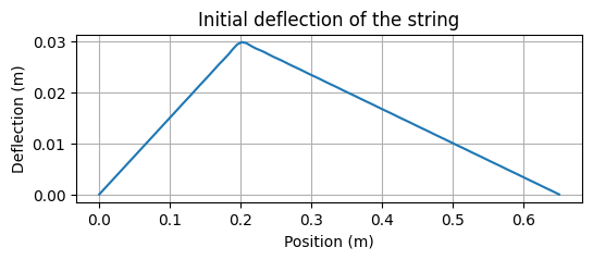
Get the initial conditions or the excitation

u0_modal = create_pluck_modal(
    lambda_mu,
    pluck_position=excitation_position,
    initial_deflection=initial_deflection,
    string_length=string_params.length,
)
u0 = inverse_STL(K, u0_modal, string_params.length)
fig, ax = plt.subplots(1, 1, figsize=(6, 2))
ax.plot(grid, u0)
ax.set_xlabel("Position (m)")
ax.set_ylabel("Deflection (m)")
ax.set_title("Initial deflection of the string")
ax.grid(True)

Get \(\gamma_{\mu}\) and \(\omega_{\mu}\) and integrate in time from the initial conditions defined above. This should be very fast, even for a large number of modes.

gamma2_mu = damping_term(
    string_params,
    lambda_mu,
)
omega_mu_squared = stiffness_term(
    string_params,
    lambda_mu,
)

modal_sol = solve_sinusoidal(
    gamma2_mu,
    omega_mu_squared,
    u0_modal,
    n_steps,
    dt,
)

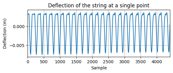
Transform the modal solution back to the physical space using the precomputed eigenfunctions, or evaluate at a single point.

mu = np.arange(1, n_modes + 1)  # mode indices

readout_weights = evaluate_string_eigenfunctions(
    mu,
    readout_position,
    string_params,
)

# at a single point
u_readout = readout_weights @ modal_sol

# at all points
sol = inverse_STL(K, modal_sol, string_params.length)

Single point:

All points:

Once Loop Reflect

Plate

We do a very similar thing for plates. First define the parameters

n_modes_x = 8
n_modes_y = 8
n_modes = n_modes_x * n_modes_y
n_steps = 44100
sample_rate = 44100
dt = 1.0 / sample_rate
excitation_duration = 1.0  # seconds
excitation_amplitude = 1.0
force_position = (0.05, 0.05)
readout_position = (0.1, 0.1)
plate_params = PlateParameters(
    Ts0=0,
    d1=4e-3,
    d3=3e-2,
)

Get the eigenpairs

wnx, wny = plate_wavenumbers(
    n_modes_x,
    n_modes_y,
    plate_params.l1,
    plate_params.l2,
)
lambda_mu_2d = plate_eigenvalues(wnx, wny)
n_gridpoints_x = 101
n_gridpoints_y = 151
x = np.linspace(0, plate_params.l1, n_gridpoints_x)
y = np.linspace(0, plate_params.l2, n_gridpoints_y)
K = plate_eigenfunctions(wnx, wny, x, y)

# Sort the eigenvalues and get the indices
indices = np.argsort(lambda_mu_2d.ravel())
ky_indices, kx_indices = np.unravel_index(indices, lambda_mu_2d.shape)
ky_indices, kx_indices = ky_indices + 1, kx_indices + 1
selected_indices = np.stack([kx_indices, ky_indices], axis=-1)
lambda_mu = np.sort(lambda_mu_2d.reshape(-1))

This time we will use an excitation force instead on initial conditions. We define the force as a 1D raised cosine at a single point on the plate.

rc = create_1d_raised_cosine(
    duration=excitation_duration,
    start_time=0.010,
    end_time=0.012,
    amplitude=excitation_amplitude,
    sample_rate=sample_rate,
)

weights_at_ex = (
    evaluate_rectangular_eigenfunctions(
        selected_indices,
        force_position,
        params=plate_params,
    )
    / plate_params.density
)

weights_at_readout = evaluate_rectangular_eigenfunctions(
    selected_indices,
    readout_position,
    params=plate_params,
)

modal_excitation = np.outer(rc, weights_at_ex)

Get \(\gamma_{\mu}\) and \(\omega_{\mu}\) and integrate in time using the excitation force.

gamma2_mu = damping_term(
    plate_params,
    lambda_mu,
)
omega_mu_squared = stiffness_term(
    plate_params,
    lambda_mu,
)


def nl_fn(modal_sol):
    return 0.0


_, modal_sol = solve_tf_excitation(
    gamma2_mu,
    omega_mu_squared,
    modal_excitation,
    dt,
    nl_fn=nl_fn,
)

Get the solution in physical space